利用离散时间系统实现连续时间系统
问题描述
利用离散时间系统实现连续时间系统。 1) 如图 (a)所示为一个连续时间系统。 2) 图 (b)为连续信号经过 AD 变换变为离散信号,通过离散时间系统,然后经过 DA 变换变为连续信号。 3) 对上述 2 种方法进行仿真比较。并探究什么时候 2 种方法的输出结果是一致的。
提示:Matlab 编程实现中都是针对的离散信号,可以用较短的时间间隔来表示连续信号,用较长的时间间隔来表示离散信号。
理论引入
在学《数字电子技术基础》的时候我们知道Nyquist-Shannon sampling theorem,当采样率至少是信号带宽的两倍,输出信号可避免重叠。那么最佳采样值可参考其进行选取。
解决方法
讨论一
先讨论简单情况,当$x(t) = \sin t$,$h(t) = \delta(t)$时,$y(t) = \sin t$
1
2
3
4
5
6
7
8
9
10
11
12
13
14
15
16
17
18
19
20
21
22
23
24
25
26
27
28
29
30
31
32
33
34
35
36
37
38
39
40
t = 0:0.001:5; % 时间范围
f = 1/2; % 信号频率
x = sin(2*pi*f*t); % 连续信号

fs = 2; % 采样率
Ts = 1/fs; % 采样周期
n = 0:Ts:5; % 离散时间范围
xd = sin(2*pi*f*n); % 离散信号

t_interp = 0:0.01:5; % 插值时间范围
y = interp1(n, xd, t_interp, 'linear'); % 线性插值

% 绘制连续信号
figure;
subplot(2,2,1);
plot(t, x);
title('Continuous Signal');
xlabel('Time');
ylabel('Amplitude');

% 进行AD转换(模拟到数字)
subplot(2,2,2);
stem(n, xd);
title('Discrete Signal (After AD Conversion)');
xlabel('Discrete Time');
ylabel('Amplitude');

% 设计离散时间系统
subplot(2,2,3);
plot(n, xd);
title('Output of Discrete-Time System');
xlabel('Discrete Time');
ylabel('Amplitude');

% 进行DA转换(数字到模拟)
subplot(2,2,4);
plot(t_interp, y);
title('Reconstructed Continuous Signal (After DA Conversion)');
xlabel('Time');
ylabel('Amplitude');
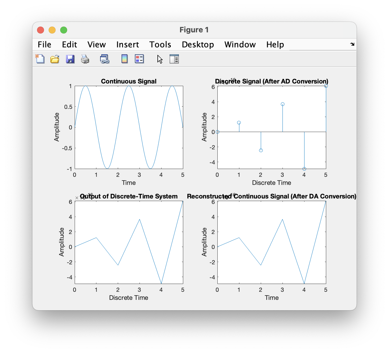
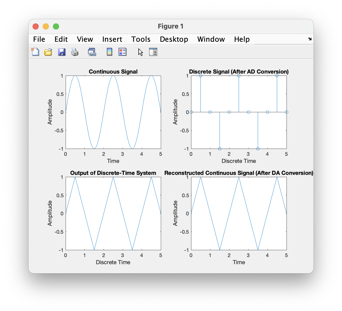
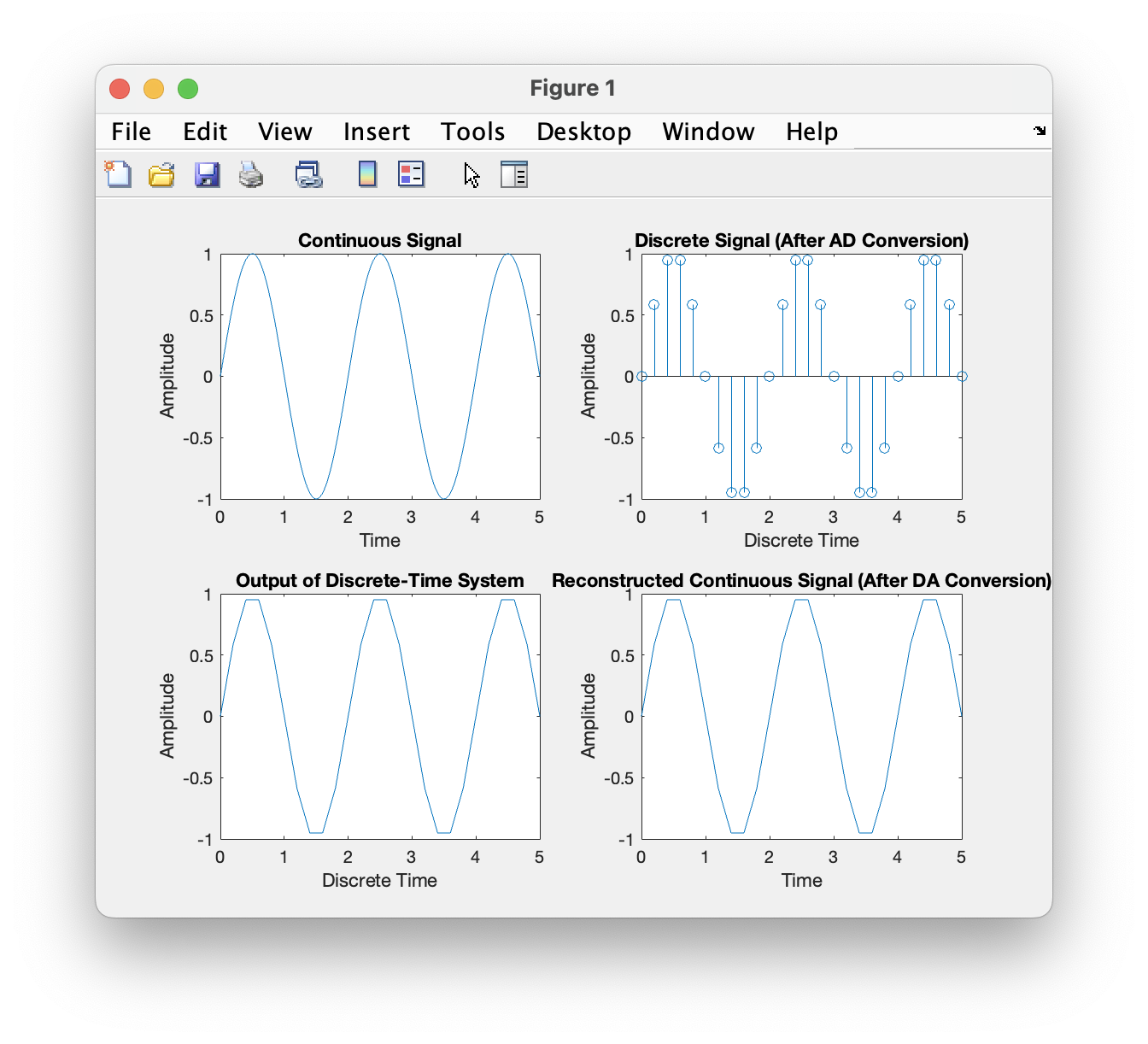
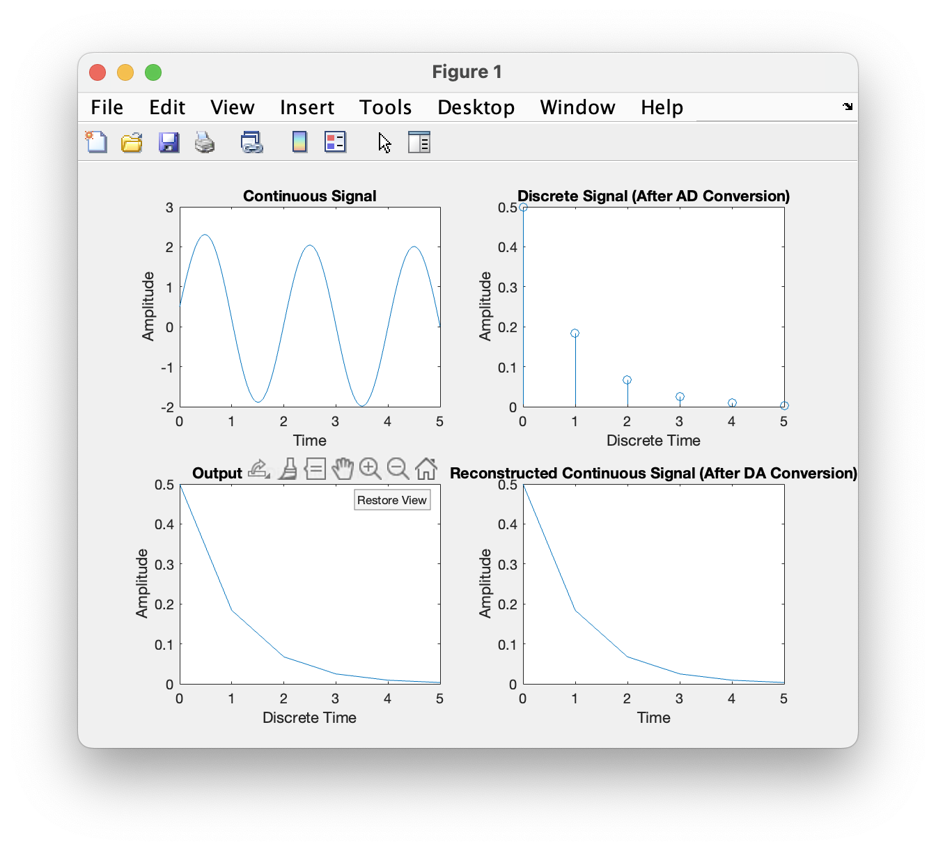
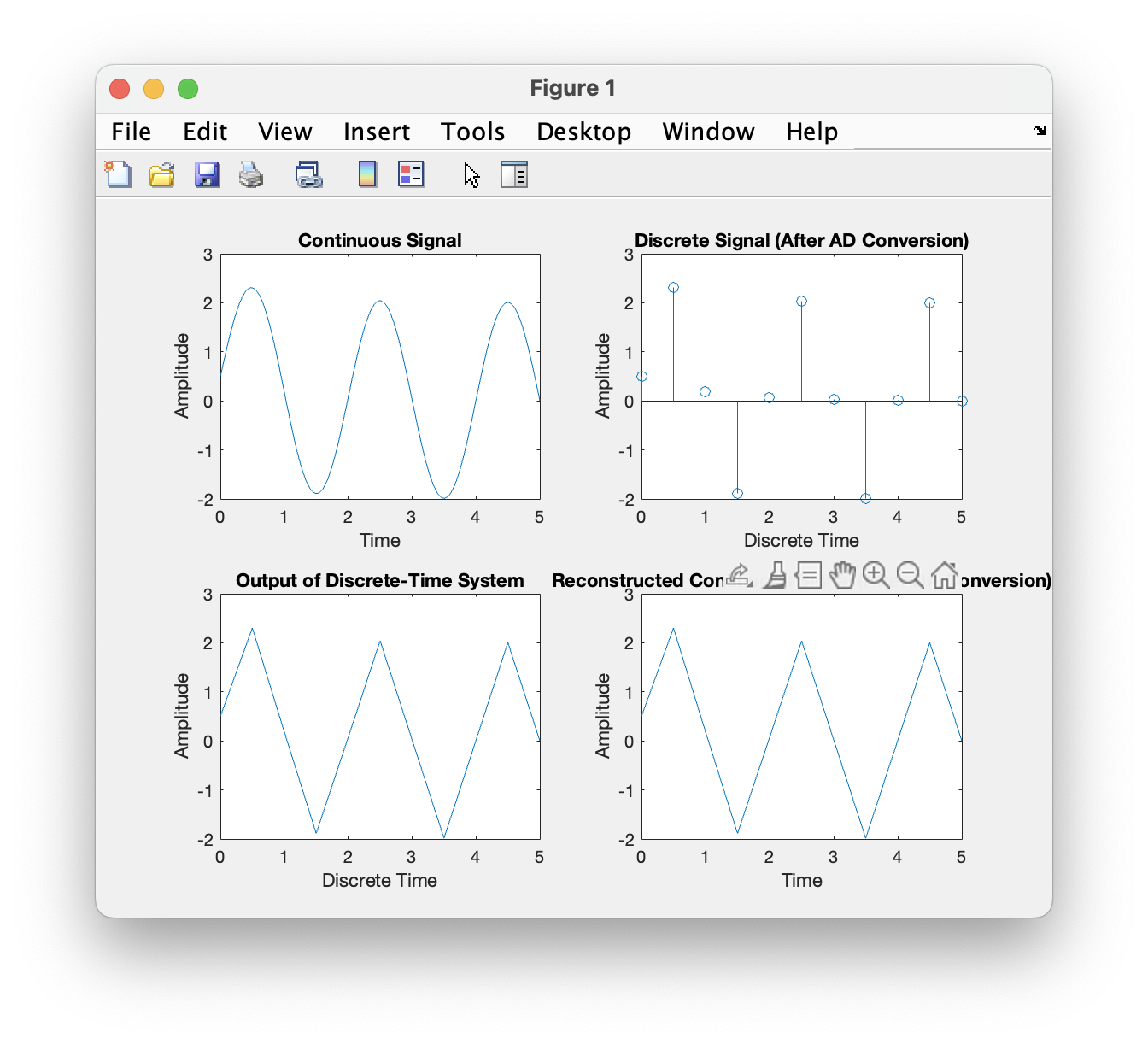
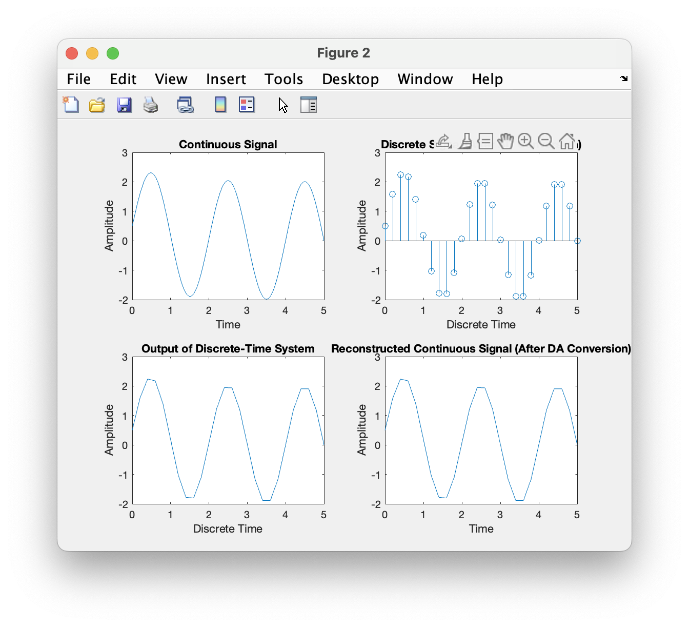
采样率为1时,输出信号严重失真,当采样率为2时其基本信息被保留下来,采样率为10时,信号还原度相对较好。
讨论二
当$h(t)$不为$\delta(t)$时,由于$y(t) = x(t) * h(t)$,卷积为线性运算,不会改变信号的频率,所以仍有:
1
2
3
4
5
6
7
8
9
10
11
12
13
14
15
16
17
18
19
20
21
22
23
24
25
26
27
28
29
30
31
32
33
34
35
36
37
38
39
40
41
42
t = 0:0.001:5; % 时间范围
f = 1/2; % 信号频率
x = sin(2*pi*f*t); % 连续信号
y = 2*x + 0.5*exp(-t);

fs = 2; % 采样率
Ts = 1/fs; % 采样周期
n = 0:Ts:5; % 离散时间范围
xd = sin(2*pi*f*n); % 离散信号
yd = 2*xd + 0.5*exp(-n);

t_interp = 0:0.01:5; % 插值时间范围
y1 = interp1(n, yd, t_interp, 'linear'); % 线性插值

% 绘制连续信号
figure;
subplot(2,2,1);
plot(t, y);
title('Continuous Signal');
xlabel('Time');
ylabel('Amplitude');

% 进行AD转换(模拟到数字)
subplot(2,2,2);
stem(n, yd);
title('Discrete Signal (After AD Conversion)');
xlabel('Discrete Time');
ylabel('Amplitude');

% 设计离散时间系统
subplot(2,2,3);
plot(n, yd);
title('Output of Discrete-Time System');
xlabel('Discrete Time');
ylabel('Amplitude');

% 进行DA转换(数字到模拟)
subplot(2,2,4);
plot(t_interp, y1);
title('Reconstructed Continuous Signal (After DA Conversion)');
xlabel('Time');
ylabel('Amplitude');
结论
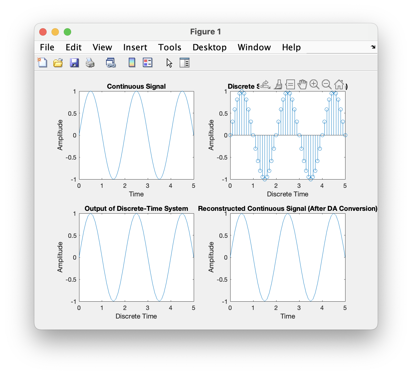
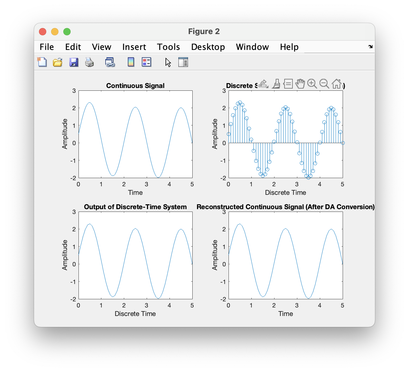
当采样率大于两倍奈奎斯特频率时,输出信号保留了原有信号的基本信息,当采样率在3倍奈奎斯特频率以上时,两种方法的输出结果几乎一直。
This post is licensed under CC BY 4.0 by the author.